Parsing mathematical equation to generate computation graphs - First step from software 1.0 to 2.0 in go
In a previous article, I described an implementation of an RNN from scratch in go. The target is to use the RNN as a processing unit. The ultimate goal is to create a portable tool cross platform and able to grab and process data where they are. I have many applications in mind such as finding the root-cause of an incident or managing the capacity of an infrastructure.
Note I stick to the Go language for many reasons: Some of them a personnal and not opposable (I simply like it). But another reason is that, in a distant future, this tool could act as a node of a processing network that would communicate via a tuple space (see my previous posts about Linda: Linda, 31yo with 5 starving philosophers, To Go and touch Linda’s Lisp and Linda’s eval/C: a tuplespace oddity.
All the node would work in a choreography. The set of nodes would be a kind of distributed bot that could monitor a complete IT system. But that’s for another story in a couple of years…
Back to 2017-2018: the purpose of this article is to describe a way to code in software 1.0 an execution machine for a software 2.0.
I will first explain the concepts. Then I will explain why a LSTM (a certain kind of neural network) is a software 2.0. Then I will describe a way to parse and execute this software 2.0 on a machine coded in Go (software 1.0).
Considerations about software 1.0 and software 2.0
What is a software?
It is a sequence of bits and bytes that can be computed, and that produces a result (the solution of a problem for example).
To build a software until now, a compiler is used. Its goal is to turn a “human readable sequence of characters”, called code, into the sequence of bytes.
This sequence of bytes is evaluated and executed by a machine at run time. Depending on the input, the execution produces (hopefully) the expected output.
The art of programming, is, in essence, the faculty for a human to describe the solution of a problem and to express it in a computer language.
What is software 2.0?
I discovered the concept of software 2.0 thanks to Andrej Karpathy’s blog. The idea is similar to any software: a compiler is used to turn a sequence of code into a sequence of bytes. This sequence is interpreted by a machine.
The difference is that the code is a sequence of mathematical equations (called model). Those equations are composed of variables and “constants”. Let’s call the constants “the weights”.
The compiler is a software 1.0 that is able to transpile the equations into a sequence of bytes that will be evaluated by a machine (note that the compiler itself is a machine).
So what is the difference between 1.0 and 2.0? Is it just a matter of language?
No, the major difference is in the art of programming and the use case.
For example:
A programmer cannot write an algorithm that will solve a specific problem (ex: I need to recognize a cat in photo).
So, the programmer will write a set of equations able to solve a kind of problem (recognize objects on any photo).
The solution to the specific problem will be given by the evaluation of the equation for a specific set of weights (a cat is an object that corresponds to the specific set of weights: for example {0,1,3,2,45,6,6,5,3,4,6,….}.)
And what makes the software 2.0 so specific? The amount of weights is so important that it cannot be determined manually. It is determined empirically. And a computer is faster than any human in this learning process.
Yes, machine learning is a discipline of software 2.0
Example of a software 2.0: Deep learning
Neural networks are the perfect representation of the software 2.0. In my last blog post I have implemented a recurrent neural network in pure go.
My toy is working, but I have been disappointed by the results: the generated text is poor and repetitive (for example it generates: hello, the the the the the the...). Vanillas RNNs are suffering from the vanishing gradient problem which is most likely the root cause of this weird behavior.
One solution is to change the core model for a more robust network called __L__ong __S__hort __T__erm __M__emory network (LSTM for short).
The software 2.0 will be an implementation of the equations of the LSTM. Form more information about LSTM, I strongly encourage you to read Understanding LSTM Networks from Christopher Olah.
LSTM
LSTM are a bit more complex than vanilla RNN. Therefore, a naive Go implementation as made for the RNN is harder to code.
As one of my goal is to understand how things deeply works (some articles such as “Yes you should understand backprop” makes me confident that it is not a waste of time).
The tricky part of the implementation is in the process called backpropagation. I have tried to implement the back propagation mechanism manually without any luck. I have search the web for an algorithm. The best explanation I have found so far is in the cs231n course from Stanford. It is a clear explanation of how the process works. And it is obvious that a graphical representation of the equations helps a lot in the computation of the gradient.
Equations are graphs
So equations are graphs…
This post from Chewxy is a perfect illustration of how the expression of a mathematical expression is turned into a graph at a compiler level.
So my software 1.0 must be made of graphs.
Writing the machinery: software 1.0
So far, we have understood that machine learning is about graphs and tensors (multidimensional arrays). It exists some optimized library to transpile the equations into graphs. Tensorflow is one of those. Tensorflow is highly optimized, but the setup of the working environment may be tricky from times to time. As of today, it is not a good candidate for my skynet robot :).
Gorgonia
The author of the post about equation I quoted previously, is also the author of the Gorgonia project.
Gorgonia is self-describe like this in its documentation:
Package Gorgonia is a library that helps facilitate machine learning in Go. Write and evaluate mathematical equations involving multidimensional arrays easily. Do differentiation with them just as easily.
This is exactly the answer to my problem.
I have talked to the author on the channel #data-science on gophers.slack.com. He is really committed, and very active. On top of that I am really attracted by the idea of such a library in go. I have decided to give Gorgonia a try.
Machines, Graphs, Nodes, Values and Backends
In Gorgonia an equation is represented by an ExprGraph. It is the main entry point of Gorgonia.
A graph is composed of Nodes.
A node is any element in the graph. It is a placeholder that will host a Value.
A Value is an interface. A Tensor is a type of Value.
Tensors are multidimensional arrays that contains elements of the same Dtype. All those elements are stored in concrete arrays of elements (for example []float32).
To actually compute the graph, Gorgonia is using “a machine”:
- a
lispMachineor - a
tapeMachine
Building a graph
Let’s see a very simple example of a Gorgonia implementation.
To transform a mathematical equation into a graph, we first need to create a graph, then create the Values, assign them to some nodes and add the nodes to the graph.
For example, this equation:
$$z = W \cdot x$$ With $$W = \begin{bmatrix}0.95 & 0,8 \\ 0 & 0\end{bmatrix}, x = \begin{bmatrix}1 \\ 1\end{bmatrix}$$
Is written like this in “Gorgonia”:
// Create a graph
g := G.NewGraph()

// Create the backend with the inputs
vecB := []float32{1,1}
// Create the tensor and specify its shape
vecT := tensor.New(tensor.WithBacking(vecB), tensor.WithShape(2))
// Create a node of type "vector"
vec := G.NewVector(g,
        tensor.Float32,    // The type of the data encapsulated within the node
        G.WithName("x"),   // The name of the node (optional)
        G.WithShape(2),    // The shape of the Vector
        G.WithValue(vecT), // The value of the node
)
matB := []float32{0.95,0.8,0,0}
matT := tensor.New(tensor.WithBacking(matB), tensor.WithShape(2, 2))
mat := G.NewMatrix(g,
        tensor.Float32,
        G.WithName("W"),
        G.WithShape(2, 2),
        G.WithValue(matT),
)

// z is a new node of the graph "g".
// It does not contains the actual result because the graph
// has not be computed yet
z, err := G.Mul(mat, vec)
// ... error handling

// create a VM to run the program on
machine := G.NewTapeMachine(g)

// The graph is executed now !
err = machine.RunAll()
// ... error handling
// Now we can print the value of z
fmt.Println(z.Value().Data())
// will display [1.75 0] which is a []float32{}
The problem is:
The more complex the model is, the more verbose the code will be, the harder to debug. For example, a LSTM with a forget gate is expressed like this:

Source: wikipedia
Transpiling it with Gorgonia will lead to something like this:
var h0, h1, inputGate *Node
h0 = Must(Mul(l.wix, inputVector))
h1 = Must(Mul(l.wih, prevHidden))
inputGate = Must(Sigmoid(Must(Add(Must(Add(h0, h1)), l.bias_i))))

var h2, h3, forgetGate *Node
h2 = Must(Mul(l.wfx, inputVector))
h3 = Must(Mul(l.wfh, prevHidden))
forgetGate = Must(Sigmoid(Must(Add(Must(Add(h2, h3)), l.bias_f))))

var h4, h5, outputGate *Node
h4 = Must(Mul(l.wox, inputVector))
h5 = Must(Mul(l.woh, prevHidden))
outputGate = Must(Sigmoid(Must(Add(Must(Add(h4, h5)), l.bias_o))))

var h6, h7, cellWrite *Node
h6 = Must(Mul(l.wcx, inputVector))
h7 = Must(Mul(l.wch, prevHidden))
cellWrite = Must(Tanh(Must(Add(Must(Add(h6, h7)), l.bias_c))))

// cell activations
var retain, write *Node
retain = Must(HadamardProd(forgetGate, prevCell))
write = Must(HadamardProd(inputGate, cellWrite))
cell = Must(Add(retain, write))
hidden = Must(HadamardProd(outputGate, Must(Tanh(cell))))
Actually the concept is close to the Reverse Polish Notation. But what would make my life easier would be to process the equation written as-is in unicode:
set(`iₜ`, `σ(Wᵢ·xₜ+Uᵢ·hₜ₋₁+Bᵢ)`)
set(`fₜ`, `σ(Wf·xₜ+Uf·hₜ₋₁+Bf)`)
set(`oₜ`, `σ(Wₒ·xₜ+Uₒ·hₜ₋₁+Bₒ)`)
set(`ĉₜ`, `tanh(Wc·xₜ+Uc·hₜ₋₁+Bc)`)
ct := set(`cₜ`, `fₜ*cₜ₋₁+iₜ*ĉₜ`)
set(`hc`, `tanh(cₜ)`)
ht, _ := l.parser.Parse(`oₜ*hc`)
Note If you don’t have the correct font to display the unicode character click to view the unicode character screenshot
Good ol’ software 1.0
What I will do is to write a lexer and a parser to analyze the mathematical equations written in unicode and generate the corresponding Gorgonia execution graph.
Lexer/Parser
My first attempt was to use a simple lexer and a simple parser. This is described in many posts over the internet all based on a talk by Rob Pike: Lexical Scanning in GO. I have been able to write the lexer easily. The parser was more difficult to write because of the mathematical operator precedence.
After a bunch of documentation about LALR parser, I have decided to call an old friend: yacc
In the world of go, there is goyacc whose syntax is compatible with yacc, but which generates parsers written in go. I have found a perfect example of a calculator in the goyacc test data
The grammar
The token that I will recognize are the basic matrix operations I need for my LSTM, plus the sigmoid and the tanh function:
%token '+' '·' '-' '*' '/' '(' ')' '=' 'σ' tanhthe yylval are always pointer to Gorgonia nodes
%union {
        node *G.Node
}

%token  <node>  NODE
The grammar and the application of the operators are all described in a couple of lines. For example, addition and multiplications are described like this:
...
expr1:
        expr2
|       expr1 '+' expr2
        {
                $$ = G.Must(G.Add($1,$3))
        }
|       expr1 '-' expr2
        {
                $$ = G.Must(G.Sub($1,$3))
        }

expr2:
        expr3
|       expr2 '·' expr3
        {
                $$ = G.Must(G.Mul($1,$3))
        }
|       expr2 '*' expr3
        {
                $$ = G.Must(G.HadamardProd($1,$3))
                        }
|       expr2 '/' expr3
        {
                $$ = G.Must(G.Div($1,$3))
        }
...
The parser and the lexer
The lexer implementation is a struct type that fulfills the interface
type yyLexer interface {
	Lex(lval *yySymType) int
	Error(e string)
}
The Lexer will read elements such as Wₜ, but will not know how to associate it with the variable that points to Gorgonia.Node.
My lexer must be aware of a correspondence between a unicode representation and the actual *Gorgonia.Node.
For this purpose, I add a dictionary of elements. It is a map whose key is the representation and the value is the pointer to the Node:
type exprLex struct {
	line []byte
	peek rune
        dico map[string]*G.Node // dictionary
	g      *G.ExprGraph
        result *G.Node
        err error
}
I also add Let method that sets an entry in the dictionary.
func (x *exprLex) Let(ident  string, value *G.Node) {
        x.dico[ident] = value
}
I will not describe the rest of the parser because the implementation is straightforward and easy to read. You can find the complete implementation in the expr.y source file.
Generating the package
This is the “pure” Go part.
The yacc tools actually generates a parser in go. I have chosen to declare it in its own package.
The command goyacc -o ../expr.go -p "Gorgonia" expr.y will generate the file expr.go which holds an implementation able to parse my unicode equations.
I have also added a couple of helpers function to avoid public methods. My Parser API is therefore simple:
type Parser
    func NewParser(g *G.ExprGraph) *Parser
    func (p *Parser) Parse(s string) (*G.Node, error)
    func (p *Parser) Set(ident string, value *G.Node)
(see godoc for more details).
Does it work ?
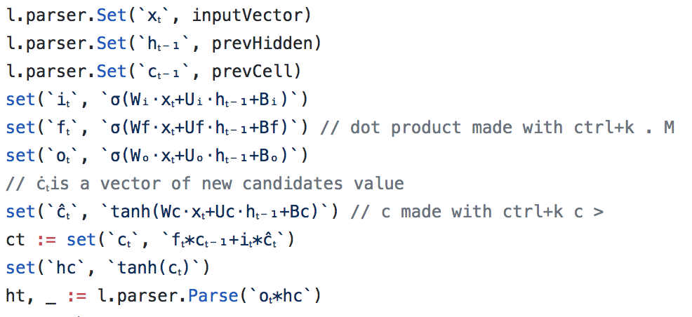
Yes ! With my parser, I am able to write a LSTM step easily and to generate an execution graph:
func (l *lstm) fwd(inputVector, prevHidden, prevCell *G.Node) (hidden, cell *G.Node) {
	// Helper function for clarity
	set := func(ident, equation string) *G.Node {
		res, _ := l.parser.Parse(equation)
		l.parser.Set(ident, res)
		return res
	}

	l.parser.Set(`xₜ`, inputVector)
	l.parser.Set(`hₜ₋₁`, prevHidden)
	l.parser.Set(`cₜ₋₁`, prevCell)
	set(`iₜ`, `σ(Wᵢ·xₜ+Uᵢ·hₜ₋₁+Bᵢ)`)
	set(`fₜ`, `σ(Wf·xₜ+Uf·hₜ₋₁+Bf)`) // dot product made with ctrl+k . M
	set(`oₜ`, `σ(Wₒ·xₜ+Uₒ·hₜ₋₁+Bₒ)`)
	// ċₜis a vector of new candidates value
	set(`ĉₜ`, `tanh(Wc·xₜ+Uc·hₜ₋₁+Bc)`) // c made with ctrl+k c >
	ct := set(`cₜ`, `fₜ*cₜ₋₁+iₜ*ĉₜ`)
	set(`hc`, `tanh(cₜ)`)
	ht, _ := l.parser.Parse(`oₜ*hc`)
	return ht, ct
}
which leads to:
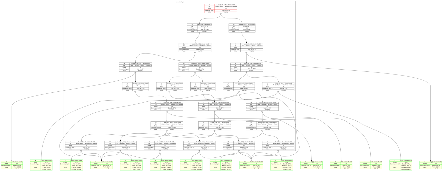
Conclusion
As Karpathy’s explained: we will still need software 1.0 to build software 2.0. I have used very old concepts to build some tools for writing and processing a software 2.0. In my example, the software 2.0 is the combination of the equations written in unicode and the values of the tensors which are arrays of floats.
A better step would be to parse a complete set of equations such as:
parse(`
iₜ=σ(Wᵢ·xₜ+Uᵢ·hₜ₋₁+Bᵢ)
fₜ=σ(Wf·xₜ+Uf·hₜ₋₁+Bf)
oₜ=σ(Wₒ·xₜ+Uₒ·hₜ₋₁+Bₒ)
ĉₜ=tanh(Wc·xₜ+Uc·hₜ₋₁+Bc)
cₜ=fₜ*cₜ₋₁+iₜ*ĉ
hₜ=oₜ*tanh(cₜ)
`)
The software 2.0, once trained, can be backed up as a unicode text file and a couple of floating point numbers. It would then be independent of the execution machine. A parser could transpile it into a Gorgonia execution graph, or a tensorflow execution graph, …
A true and independent software 2.0.
“A journey of a thousand miles must begin with a single step.” – Lao Tzu